See the guide for this topic.

1.1 – Measurements in physics

• Fundamental and derived units

Fundamental SI units

Quantity	SI unit	Symbol
Mass	Kilogram	kg
Distance	Meter	m
Time	Second	s
Electric current	Ampere	A
Amount of substance	Mole	mol
Temperature	Kelvin	K

Derived units are combinations of fundamental units. Some examples are:

• m/s (Unit for velocity)
• N (kg*m/s^²⁾ (Unit for force)
• J (kg*m^2/s^2) (Unit for energy)

• Scientific notation and metric multipliers

In scientific notation, values are written in the form a*10^n, where a is a number within 1 and 10 and n is any integer. Some examples are:

• The speed of light is 300000000 (m/s). In scientific notation, this is expressed as 3*10^8
• A centimeter (cm) is 1/100 of a meter (m). In scientific notation, one cm is expressed as 1*10^-2 m.

Metric multipliers

Prefix	Abbreviation	Value
peta	P	10^15
tera	T	10^12
giga	G	10^9
mega	M	10^6
kilo	k	10^3
hecto	h	10^2
deca	da	10^1
deci	d	10^-1
centi	c	10^-2
milli	m	10^-3
micro	μ	10^-6
nano	n	10^-9
pico	p	10^-12
femto	f	10^-15

• Significant figures

For a certain value, all figures are significant, except:

1. Leading zeros
2. Trailing zeros if this value does not have a decimal point, for example:

• 12300 has 3 significant figures. The two trailing zeros are not significant.
• 012300 has 5 significant figures. The two leading zeros are not significant. The two trailing zeros are significant.

When multiplying or dividing numbers, the number of significant figures of the result value should not exceed the least precise value of the calculation.

The number of significant figures in any answer should be consistent with the number of significant figures of the given data in the question.

FYI

• In multiplication/division, give the answer to the lowest significant figure (S.F.).
• In addition/subtraction, give the answer to the lowest decimal place (D.P.).

• Orders of magnitude

Orders of magnitude are given in powers of 10, likewise those given in the scientific notation section previously.

Orders of magnitude are used to compare the size of physical data.

Distance	Magnitude (m)	Order of magnitude
Diameter of the observable universe	10^26	26
Diameter of the Milky Way galaxy	10^21	21
Diameter of the Solar System	10^13	13
Distance to the Sun	10^11	11
Radius of the Earth	10^7	7
Diameter of a hydrogen atom	10^-10	10
Diameter of a nucleus	10^-15	15
Diameter of a proton	10^-15	15
Mass	Magnitude (kg)	Order of magnitude
The universe	10^53	53
The Milky Way galaxy	10^41	41
The Sun	10^30	30
The Earth	10^24	24
A hydrogen atom	10^-27	-27
An electron	10^-30	-30

Time	Magnitude (s)	Order of magnitude
Age of the universe	10^17	17
One year	10^7	7
One day	10^5	5
An hour	10^3	3
Period of heartheart	10^0	0

• Estimation

Estimations are usually made to the nearest power of 10. Some examples are given in the tables in the orders of magnitude section.

1.2 – Uncertainties and errors

• Random and systematic errors

Random error	Systematic error
Ÿ   Caused by fluctuations in measurements centered around the true value (spread). Ÿ   Can be reduced by averaging over repeated measurements. Ÿ  Not caused by bias.	Ÿ   Caused by fixed shifts in measurements away from the true value.Ÿ   Cannot be reduced by averaging over repeated measurements. Ÿ  Caused by bias.
Examples: Ÿ   Fluctuations in room temperature Ÿ   The noise in circuits Ÿ   Human error	Examples: Ÿ   Equipment calibration error such as the zero offset error Ÿ   Incorrect method of measurement

• Absolute, fractional and percentage uncertainties

Physical measurements are sometimes expressed in the form x±Δx. For example, 10±1 would mean a range from 9 to 11 for the measurement.

Absolute uncertainty	Δx
Fractional uncertainty	Δx /x
Percentage uncertainty	Δx/x*100%

Calculating with uncertainties

Addition/Subtraction	y=a±b	Δy=Δa+Δb (sum of absolute uncertainties)
Multiplication/Division	y=a*b or y=a/b	Δy/y=Δa/a+Δb/b (sum of fractional uncertainties)
Power	y=a^n	Δy/y=|n|Δa/a (|n| times fractional uncertainty)

• Error bars

Error bars are bars on graphs which indicate uncertainties. They can be horizontal or vertical with the total length of two absolute uncertainties.

• Uncertainty of gradient and intercepts

Line of best fit: The straight line drawn on a graph so that the average distance between the data points and the line is minimized.

Maximum/Minimum line: The two lines with maximum possible slope and minimum possible slope given that they both pass through all the error bars.

The uncertainty in the intercepts of a straight line graph: The difference between the intercepts of the line of best fit and the maximum/minimum line.

The uncertainty in the gradient: The difference between the gradients of the line of best fit and the maximum/minimum line.

1.3 – Vectors and scalars

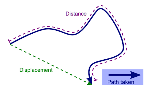
• Vector and scalar quantities

Scalar	Vector
A quantity which is defined by its magnitude only.	A quantity which is defined by both is magnitude and direction.
Examples: Ÿ   Distance Ÿ   Speed Ÿ   Time Ÿ   Energy	Examples: Ÿ   Displacement Ÿ   Velocity Ÿ   Acceleration Ÿ   Force

 

• Combination and resolution of vectors

Vector addition and subtraction can be done by the parallelogram method or the head to tail method. Vectors that form a closed polygon (cycle) add up to zero.

When resolving vectors in two directions, vectors can be resolved into a pair of perpendicular components.

FYI

The relationship between two sets of data can be determined graphically.

Relationship	Type of Graph	Slope	y-intercept
y=mx+c	y against x	m	c
y=kx^n	logy against logx	n	logk
y=kx^n+c with n given	y against x^n	k	c